Back to Kemp Acoustics Home


Next: Solutions for a cylinder
Up: Multimodal propagation in acoustic
Previous: Plane waves at a
Contents
The inclusion of higher modes in horn acoustics has been
studied recently [32,33,38,41,42].
In general, the
pressure and velocity in a cylinder can be expressed in terms of the
modes of the duct whose
amplitude patterns have  nodal circles and
  nodal diameters on a
circular cross-section where
nodal diameters on a
circular cross-section where  is the plane wave mode.
We are analysing axi-symmetric systems so we will treat axi-symmetric
(nodal circle) modes only. The pressure and volume velocity are then vectors
with a single subscript, .
is the plane wave mode.
We are analysing axi-symmetric systems so we will treat axi-symmetric
(nodal circle) modes only. The pressure and volume velocity are then vectors
with a single subscript, .
In the case of rectangular cross-section, the
modes of the duct will have an integer number of nodal lines parallel to the
 axis and an integer number of nodal lines parallel to the
  axis.
We will only treat systems that preserve symmetry about the central axis, so
only modes with an even number of nodal lines in both dimensions need to be
considered and the subscript
axis.
We will only treat systems that preserve symmetry about the central axis, so
only modes with an even number of nodal lines in both dimensions need to be
considered and the subscript  will be used where
there are
will be used where
there are  nodal lines parallel to the axis and
  nodal lines
parallel to the axis.
nodal lines
parallel to the axis.
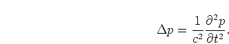
The pressure for each mode obeys the 3
dimensional wave equation:
 |
(2.22) |
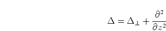
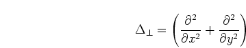
Here  is the Laplacian operator which may be expressed as the sum
of the
is the Laplacian operator which may be expressed as the sum
of the  direction component and the component on the - plane:
 |
(2.23) |
where  is given in Cartesian coordinates as
 |
(2.24) |
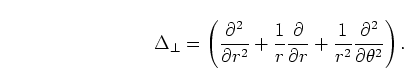
and in cylindrical polars as
 |
(2.25) |
The wave equation can be solved by expressing the pressure as a sum of
the contributions of the modes of the duct where each term is
the multiplication of the profiles along ,  and the - plane.
We can then solve the problem by separation of
variables ([43] pp.540-556).
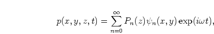
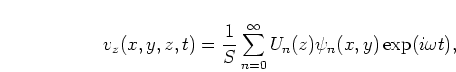
From Pagneux et al. [32] the pressure and axial velocity are:
 |
(2.26) |
 |
(2.27) |
where  is the pressure profile on the - plane and
  is the pressure profile of the th mode along the length of the tube.
Similarly,
is the pressure profile of the th mode along the length of the tube.
Similarly,  is the axial volume velocity profile of the
th mode along the length of the tube. and are in general
complex numbers to take phase into account.
Note that although it is convenient to refer to as the volume
velocity, the net volume velocity is
is the axial volume velocity profile of the
th mode along the length of the tube. and are in general
complex numbers to take phase into account.
Note that although it is convenient to refer to as the volume
velocity, the net volume velocity is  ; the other
entries are the amplitudes of the axial velocity distributions multiplied by
the surface area but have no net contribution to the volume
velocity [32].
; the other
entries are the amplitudes of the axial velocity distributions multiplied by
the surface area but have no net contribution to the volume
velocity [32].
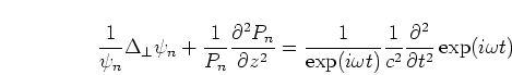
Equation (2.26) gives the pressure as a series of terms,  being unity, and so the
  contribution represents plane wave propagation
while the other modes have a non-uniform pressure profile. Substituting
contribution represents plane wave propagation
while the other modes have a non-uniform pressure profile. Substituting
 from equation (2.26) into the wave
equation (2.22) and dividing through by gives:
from equation (2.26) into the wave
equation (2.22) and dividing through by gives:
 |
(2.28) |
Since each term in this equation is a function of a different variable, each
term must equal a constant.
The differentiation with respect to is straightforward giving
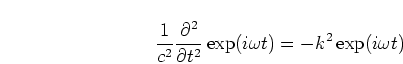 |
(2.29) |
with the eigenvalue  being the free space wavenumber.
Defining
being the free space wavenumber.
Defining  to be the wavenumber along (commonly referred to as the
propagation factor):
to be the wavenumber along (commonly referred to as the
propagation factor):
 |
(2.30) |
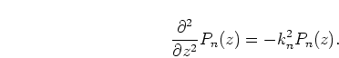
The transverse term gives
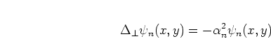 |
(2.31) |
with  being the eigenvalue of the th mode. Physically
is the wavenumber in the - plane and is zero for plane wave propagation
and is positive and real for the modes which feature nodal lines or circles.
being the eigenvalue of the th mode. Physically
is the wavenumber in the - plane and is zero for plane wave propagation
and is positive and real for the modes which feature nodal lines or circles.
It then follows from equation (2.28) that the
wavenumbers follow the relation
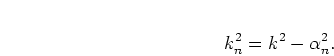 |
(2.32) |
The wavelength along will be
 .
.
Note that in a pipe of uniform cross-section the solution of equation
(2.30) gives
 |
(2.33) |
To find the corresponding volume velocities we use the force equation
(2.4). The component of the velocity is
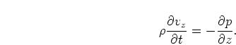 |
(2.34) |
giving the corresponding axial volume velocity as
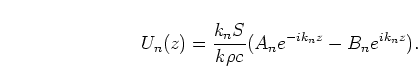 |
(2.35) |
We can note from this that the characteristic
impedance, defined to be the ratio of pressure and volume velocity of
forward travelling waves, also depends on the mode number, . For plane
waves it was
 but for the th mode this becomes:
 |
(2.36) |
Assuming loss-less propagation is positive and real above cut-off
point (
 ) so the pressure varies sinusoidally along the axis
with a wavelength of
) so the pressure varies sinusoidally along the axis
with a wavelength of
 where
where
 is the
free-space wavelength.
Below the cut-off point is negative and imaginary [42]
so the pressure will be exponentially damped. Calculation of
first requires calculation of which in turn
depends on the boundary conditions in equation (2.31)
(and therefore on the geometry of the duct). It will
be treated for both lossy and non-lossy propagation in section
2.4.1 for ducts of circular cross-section and in section
2.4.2 for rectangular ducts.
is the
free-space wavelength.
Below the cut-off point is negative and imaginary [42]
so the pressure will be exponentially damped. Calculation of
first requires calculation of which in turn
depends on the boundary conditions in equation (2.31)
(and therefore on the geometry of the duct). It will
be treated for both lossy and non-lossy propagation in section
2.4.1 for ducts of circular cross-section and in section
2.4.2 for rectangular ducts.
We have seen that plane waves travelling across a section of tube are only
reflected when the cross-section changes.
The plane wave pressure amplitude at any point in a uniform section of tube
may be obtained from a known plane wave pressure amplitude at a single point
simply by projection using equation (2.10). Each of the other modes of
the pipe will also
only be reflected where the cross-section changes and so may be treated
independently in a section of uniform cross-section. The wavenumber along
the axis becomes for the th mode and, as discussed earlier in the
section, the characteristic
impedance of the th mode is
 .
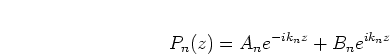
Projection of pressure and volume velocity complex amplitudes
of the th mode then follow from equations (2.10) and (2.11).
.
Projection of pressure and volume velocity complex amplitudes
of the th mode then follow from equations (2.10) and (2.11).
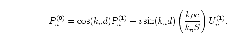 |
(2.37) |
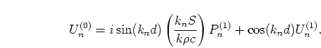 |
(2.38) |
Here  and
and  are the complex amplitudes of the pressure
and volume velocity of the th mode on plane 0 and
are the complex amplitudes of the pressure
and volume velocity of the th mode on plane 0 and  and
and
 are the complex amplitudes of the pressure and volume velocity
of the th mode on plane 1 with the planes separated by a distance
are the complex amplitudes of the pressure and volume velocity
of the th mode on plane 1 with the planes separated by a distance  (see figure 2.1).
We define the pressure vector,  , as a column vector consisting of
the modal pressure amplitudes
, as a column vector consisting of
the modal pressure amplitudes  and
and
 as a column vector of the corresponding
  values.
A method of projecting the pressure and velocity vectors along a uniform
section of tube will now be discussed.
values.
A method of projecting the pressure and velocity vectors along a uniform
section of tube will now be discussed.
In matrix notation the pressure vector on plane 0 is given in terms of the
vectors on plane 1 by
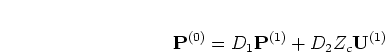 |
(2.39) |
where  ,
,  and
and  are diagonal matrices with the elements given by
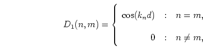 |
(2.40) |
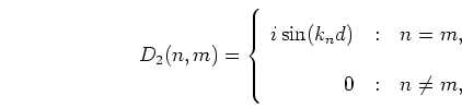 |
(2.41) |
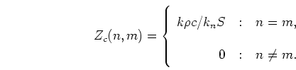 |
(2.42) |
Similarly the volume velocity on plane 0 is given in terms of the vectors
on plane 1 as
 |
(2.43) |
Subsections
Back to Kemp Acoustics Home
Next: Solutions for a cylinder
Up: Multimodal propagation in acoustic
Previous: Plane waves at a
Contents
Jonathan Kemp
2003-03-24