Back to Kemp Acoustics Home


Next: Acoustic pulse reflectometry measurement
Up: Maximum length sequences
Previous: Auto-correlation property of MLS
Contents
The frequency content of the signal recorded at the microphone will contain
information on the frequency response of the system under test. In order to
go beyond this and get the impulse response of the system, we must use the
auto-correlation property of the MLS signals. First recognise that the
measured signal is the convolution of the MLS and the system impulse response.
We will define the input impulse response of our system as  . We will refer
to as the system impulse response to prevent confusion with the input
impulse response of a pulse reflectometry test object. This distinction will
be discussed in more detail in section 7.5.4. The MLS signal is
. We will refer
to as the system impulse response to prevent confusion with the input
impulse response of a pulse reflectometry test object. This distinction will
be discussed in more detail in section 7.5.4. The MLS signal is  ,
so the pressure,
,
so the pressure,  , measured at the microphone will be
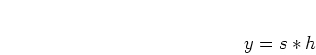 |
(7.8) |
where  here denotes convolution.
Performing correlation with respect to on both sides of equation
(7.8) gives [70]:
here denotes convolution.
Performing correlation with respect to on both sides of equation
(7.8) gives [70]:
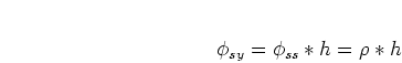 |
(7.9) |
where  is notation for the correlation of
  and
and  . Note
that convolution in the time domain is multiplication in the frequency domain,
so the fact that the frequency spectrum of
. Note
that convolution in the time domain is multiplication in the frequency domain,
so the fact that the frequency spectrum of  is flat, except for the zero
frequency component, means that is left unchanged by convolution with
except for a small dc offset of the order of
is flat, except for the zero
frequency component, means that is left unchanged by convolution with
except for a small dc offset of the order of  . The
impulse response of the system
can therefore be extracted from the measurement of the system response by
correlation with the MLS input. Correlation is defined as
. The
impulse response of the system
can therefore be extracted from the measurement of the system response by
correlation with the MLS input. Correlation is defined as
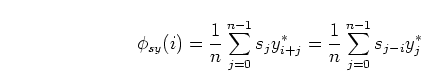 |
(7.10) |
which can be converted to a matrix notation by making a matrix  consisting of
  circularly shifted versions of [70]:
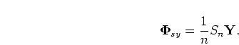 |
(7.11) |
The elements of are given by
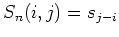 where
where  is taken
modulo so that the successive rows of the matrix contain shifted
one step to the right each time with the values leaving on the right
appearing on the left.
is taken
modulo so that the successive rows of the matrix contain shifted
one step to the right each time with the values leaving on the right
appearing on the left.
 is a column vector of the measured system response and
 a column vector of the resulting correlation.
The cross-correlation can also be performed in the frequency domain by
considering the close relationship between cross-correlation and convolution.
Deconvolution was performed by frequency domain division in chapter
5. Convolution on the other hand may performed by
multiplication in the frequency domain.
Cross-correlation of two signals is the reverse of the
first sequence convolved with the second sequence [59] pp.92-96:
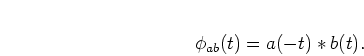 |
(7.12) |
Reversal in the time domain means complex conjugation in the frequency domain:
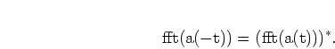 |
(7.13) |
It therefore follows that the cross-correlation of two signals in the time
domain becomes the conjugate of the first signal multiplied by the second
signal in the frequency domain.
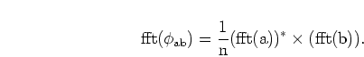 |
(7.14) |
Discrete Fourier transforms are used for the analysis in this chapter. The
speed of analysis is acceptable for the measurements we present here.
Before acceptable computational power was available, it was necessary to
perform
interpolation to make the length of the sequence up to  , enabling
the use of fast Fourier transforms [66]. Another option
is the fast Hadamard transform technique as set out in Borish and Angell
[70] which does not require interpolation and is less computationally
expensive.
, enabling
the use of fast Fourier transforms [66]. Another option
is the fast Hadamard transform technique as set out in Borish and Angell
[70] which does not require interpolation and is less computationally
expensive.
Back to Kemp Acoustics Home
Next: Acoustic pulse reflectometry measurement
Up: Maximum length sequences
Previous: Auto-correlation property of MLS
Contents
Jonathan Kemp
2003-03-24