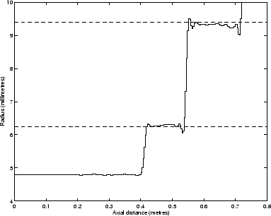
The step up from the dc tube and coupler radius of 4.8 mm to the test object cylindrical section of radius of 6.25 mm is spread over a distance of 2 cm along the axis of the bore reconstruction when in reality the bore stepped up sharply. The reason for this spread is that the input impulse response measurement has a limited bandwidth; there were no significant components of the measured input impulse response above about 10 kHz because losses in the source tube damped out high frequency information in the pulse before it was able to enter the object under test. Removing the high frequencies in the impulsive reflection from a step widens the pulse, hence the algorithm interprets the reflections as coming from a more gradual expansion. The behaviour is also an example of Gibb's phenomenon [6]. When a sharp step is represented as a set of frequency components, if the high frequencies are removed, the resulting step will be oscillatory such that the filtered version is too low on the lower side of the step and over shoots to be too high at the higher side [55] pp.601-603. This effect can be more clearly seen in the step from 6.25 mm to 9.4 mm. Here the over shoot and under-shoot in the bore reconstruction is about 0.3 mm.
Within the cylindrical sections, the bore reconstruction oscillates with an amplitude of less than 0.1 mm. The average value during each cylindrical section is accurate to 0.1 mm, with the largest error at the open end of the object. In the bore reconstruction algorithm, the cross-section at each point is worked out as a fraction of the cross-section at the previous point. Hence errors accumulate as the reconstruction continues. The object chosen for measurement was useful for a test of the accuracy of the technique.
Actual musical instruments tend to have more smoothly varying bores so preventing problems due to Gibb's phenomenon. The typical accuracy of 0.1 mm for short objects has recently been successfully used to aid a manufacturer to distinguish between different trumpet leadpipes [56].
The theory in this chapter all assumed plane wave propagation in the object under test. We will see in later examples that this means that the bore reconstruction algorithm will produce errors in tubes with a large flare rate. In the following chapter we will go on to study the reflection of sound when multimodal effects are taken into account and consider how these effects might be included in a bore reconstruction algorithm.