Results

Graphs of the radiation impedance at a circular opening in an infinite baffle were produced by performing the numerical integration in equation (3.25) for a number of dimensionless frequencies ($kR$). In order to keep the general applicability of the results, as is standard practice, we will normalise the radiation impedance by dividing through by $\rho c / S$ rather than choosing a particular value of $S=\pi R^2$. Remembering that the radiation impedance is a matrix whose element $Z_{nm}$ gives the pressure amplitude of the $n$th mode due to a given volume velocity amplitude of the $m$th mode, it is useful to distinguish between the $n = m$ and $n \neq m$ elements. The $n = m$ elements are referred to as direct impedances since they give the contribution to a pressure mode by the velocity mode with the same amplitude distribution.

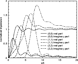
Figure 3.2 shows the real and imaginary parts of the first three direct radiation impedances for a cylindrical opening in an infinite baffle. The real part is known as the radiation resistance and a large positive value for this indicates that acoustic energy is radiated efficiently from the opening. The imaginary part is called the radiation reactance and a positive value for this indicates a mass loading of the air column [40] pp.191-192, or equivalently a length correction [45] pp.180-181. At low enough frequency the radiation impedance is effectively zero. In this case, no matter how large the velocity amplitude is, no pressure is produced, indicating the presence of a pressure node at the open end. The ideal open end condition then holds.

At low frequencies, $ka<<1$ and the impedance is small and imaginary. The very low radiation resistance means that almost no sound is radiated from the instrument. Nearly all the sound is reflected back down the tube. The small imaginary value of the impedance means that the velocity produces a small pressure, 90 degrees out of phase in the time domain, as is the case close to a pressure node in a tube supporting standing waves. A pressure node is therefore present, but has been shifted slightly from the end of the tube, which is why a correction must be made to the tube length when calculating the length of the standing waves.

At intermediate frequencies the resistance becomes larger than the reactance. The oscillatory look of all the graphs which follow in this chapter result from local maxima which occur as the wavelength becomes comparable with the tube width. In the high frequency limit the radiation impedance converges to the real value 1 (or $\rho c / S$ before normalisation) which is the characteristic impedance of plane waves in free space. This indicates that the waves are not reflected at the opening, but propagate out of the tube undisturbed and with 100% efficiency. This agrees with the intuitive behaviour of wave diffraction from an opening; high frequency waves are transmitted in a beam of the same cross-section as the opening. Standing waves cannot be set up in this regime as no energy is reflected back to contribute to resonance.

Note how the direct impedances of the modes converge more slowly as $n$ increases. The normalised characteristic impedance of the mode $n$ from equation (2.36) is $k / k_n$ which tends to 1 from above when $kR>>\gamma_n$. It is therefore observed that the radiation impedance tends to the characteristic impedance termination value, which in turn tends to 1, more slowly as $n$ (and therefore $\gamma_n$) increases.

Next we consider the elements of the impedance matrix for which $m \neq n$. These are referred to as coupled impedances since they give the contribution to a pressure mode by a velocity mode with a different amplitude distribution. Figure 3.3(a) shows the radiation impedance resulting from the coupling of the plane wave pressure mode ($n = 0$) and the $m$th velocity mode for $m=1$ and $m=2$. Figure 3.3(b) shows the radiation impedance resulting from the coupling of the pressure mode with one nodal circle ($n = 1$) and the $m$th velocity mode for $m=0$ and $m=2$.

At the zero frequency limit, the coupled radiation impedances go to zero, indicating that there is no component of the $n$th pressure mode due to the $m$th velocity mode and therefore no coupling for $kR<<1$. At intermediate frequencies we can see non-zero impedance terms (less in magnitude than for direct impedances) which indicate a certain amount of inter-modal coupling is taking place. In the high frequency limit we observe the radiation impedance tending to zero. The infinite pipe termination or characteristic impedance condition has no inter-modal coupling, or equivalently the $m \neq n$ elements of the characteristic impedance matrix have a value of zero. The radiation impedance matrix therefore tends to the characteristic impedance matrix at high frequencies for all elements, for those with $n \neq m$ in addition to those with $n = m$ discussed earlier.

Figure 3.2: Normalised direct radiation impedance of the $n$th mode in a circular duct of radius $R$ for $n=0,1,2.$

Figure 3.3: Coupled radiation impedances of a circular duct of radius R