Input impedance from the input impulse
response

We will use the theory of plane wave propagation as set out at the start of chapter 2 for the analysis which follows in this chapter. The possibility of including higher mode effects in the analysis will be discussed in chapter 7.

The pressure at the input to a tubular object will be the sum of the forward and backward going waves from equations (5.1) and (5.2):

$$p^{(1)}[nT] = \delta[nT] + iir[nT].$$ (5.3)

Similarly, the volume velocity follows from equation (2.7), giving

$$U^{(1)}[nT] = \frac{S}{\rho c} (\delta[nT] - iir[nT]).$$ (5.4)

The input impedance is defined as the ratio of the pressure and volume velocity at the input plane. So far we have obtained a time domain expression for the pressure and volume velocity if the input impulse response is known. The input impedance is generally frequency dependent however, so we must take the Fourier transform of the signals and divide the frequency components to get the input impedance at a particular frequency. The Fourier transform of an impulse is 1 for all frequencies. We define $IIR(\omega)$ as the Fourier transform of $iir[nT]$. The Fourier transform of the pressure is then

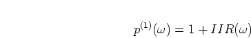$$p^{(1)}(\omega) = 1+IIR(\omega)$$ (5.5)

and the volume velocity is

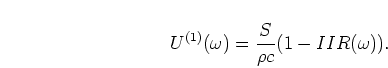$$U^{(1)}(\omega) = \frac{S}{\rho c}(1-IIR(\omega)).$$ (5.6)

Dividing in the frequency domain gives the input impedance as

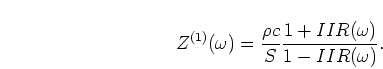$$Z^{(1)}(\omega) = \frac{\rho c}{S} \frac{1+IIR(\omega)}{1-IIR(\omega)}.$$ (5.7)

This equation lets us easily calculate the input impedance of an object once the input impulse response is obtained by measurement. Since it is impossible to produce a perfect impulse, measurement of the input impulse response is not a straight forward task and will be discussed later in the chapter. For now we proceed with the background theory to pulse reflectometry.